The Hierarchical Softmax

The Hierarchical Softmax is useful for efficient classification as it has logarithmic time complexity in the number of output classes, $log(N)$ for $N$ output classes. This utility is pronounced in the context of language modelling where words must be predicted over time steps to generate a sentence, for example, by a decoder that selects them from a vocabulary which could be in the order of $\vert \mathbf{V} \vert = 30,000$.

Small additions or modifications to the end of the article will be made when time allows in order to include remarks on use of Huffman coding with the Hierarchical Softmax and to draw links between the concepts introduced here and, for example, Noise Contrastive Estimation (NCE). This was was written on 29th March 2021, though published later.

The softmax classifier, which generalises logistic regression from a binary, $\{0 \vert 1\}$, model output to any arbitrary number of output classes, is computed by passing the so-called logit scores through the softmax function.

Given a vector of logit scores, $\mathbf{z}$, the elements are exponentiated in the numerator to make them strictly positive and divided by the sum of this exponentiation over all elements to normalise the output vector to $1$, rendering it a valid probability distribution.

The softmax should arguably be called the softargmax as it computes a smooth approximation to the $\argmax$ function, not the $\max$. The smooth property makes the function differentiable and therefore useful in neural networks as training can be done via reverse-mode automatic differentiation, specifically backpropagation [1].

Remark on Energy and the Boltzmann Distribution

It is interesting to note that the softmax is identical to the Boltzmann distribution where $z_i$ corresponds to $-\epsilon_i / kT$ and $\epsilon_i$ is a state’s energy. The distribution is defined

Here $k$ is the Boltzmann constant, a physical constant relating the average relative kinetic energy of particles in a gas with the thermodynamic temperature of that gas that is largely specific to statistical mechanics. However, $T$, which represents the thermodynamic temperature, is a commonly tweaked hyperparameter used in machine learning applications as it controls the entropy of the output distribution. Higher temperatures increase the entropy, distributing probability mass over more classes such that the softmax becomes the $\argmax$ in the limit as temperature goes to zero: ${\sigma}_T(\mathbf{z}) \rightarrow \argmax \mathbf{z}$ for $T \rightarrow 0$.

The fact that energy can be related to probabilities via the Boltzmann distribution is worth remembering in the context of Energy-Based Models (EBMs) [2].

Classification problems occur in language when models must generate probability distributions over a vocabulary of words, for example to predict the next word in language modelling. Typical vocabulary sizes could be around $30,000$.

When constructing language models, we might employ recurrent neural networks¹1 See Chris Olah’s fantastic blog post, Understanding LSTM Networks [13], for an explanation of long short-term memory networks, the most widely-used variant of RNNs, which uses gating to overcome the vanishing gradient problem. (RNNs) or transformer-based architectures²2 Read the seminal Vaswani et al. (2017) Attention is All You Need [14] for full details, Jay Alammar’s The Illustrated Transformer [15] for a readable explanation or The Annotated Transformer [16] for details on implementation. . In this case, the logit scores would be computed using a similarity score between the final layer output, $h$, and the each of the word embeddings, $v_{w_i}$.

Remark on Similarity Scores

A common choice for similarity is the dot product, $h \cdot v_{w_i}$, which is equivalent to the cosine similarity for normalised vectors (i.e. of unit norm: $\Vert x \Vert_2 = 1$). Other choices exist like the scaled dot product, $(h \cdot v_{w_i}) / d$ where $d$ is a scalar³3 In their seminal paper on Transformers, Ashish Vaswani and colleagues used scaled dot-product attention with $\sqrt{d_k}$, where $d_k$ is the feature size of the keys, to prevent the dot products from growing in magnitude thus pushing the softmax values to regions where the gradients are small and learning via backpropagation is difficult. See section 3.2.1 in Vaswani et al. (2017) Attention is All You Need [14]. , the general dot product $h \cdot W \cdot v_{w_i}$, with $W$ a matrix that permits differing dimensionality of $h$ and $v_{w_i}$ and others⁴4 See Pascale Poupart’s lecture [17] for a nice explanation. .

For the very large numbers of output classes encountered in language modelling, the softmax becomes very computationally expensive as, in order to compute the probability of any single word being the next word in a sequence, we have to compute the denominator. The denominator is linear in the feature dimensionality as it is in effect the sum of elements after a matrix-vector multiplication between the word embedding matrix and the final layer output, $\mathbf{V} \cdot h$. It is linear in the vocabulary size, $V$.

Hierarchical Softmax

Frederic Morin and Yoshua Bengio (2005) [3] proposed the hierarchical softmax classifier, an approximation to the softmax which is logarithmic-time in the vocabulary size, $\mathcal{O}(log \vert V \vert)$ in place of $\mathcal{O}(\vert V \vert)$, yielding an exponential speed-up by a factor of $\mathcal{O}(\frac{\vert V \vert}{log\vert V \vert})$.

The basic idea is to form a hierarchical description of a word as a sequence of $\mathcal{O}(log \vert V \vert)$ decisions, and to learn to take these probabilistic decisions instead of directly predicting each word’s probability. [3]

They extend the idea of Goodman [4] to define a clustering partition, $K$, of words in the vocabulary and calculate the conditional probability of a word given its context via the chain rule. In other words, for word $w$ and context $c$, with $k(.)$ a mapping from words to clusters, instead of directly computing $P(W = w \vert C = c)$, instead decompose this as

They also note that generalization could be better for choices of word clusters that “make sense”, i.e. those for which it easier to learn the second term, $P(K=k(w) \vert C = c)$. We’ll see momentarily how clusters making sense is analogous to the notion of order in lists which we can search with binary search.

They follow this up with a concrete example⁵5 I have tweaked the quote slightly to align it with the notation I introduced.

If $W$ can take $10,000$ values and we have $100$ classes [clusters] with $100$ words $w$ in each class, then instead of doing normalization over $10,000$ choices we only need to do two normalizations, each over $100$ choices. [3]

Performing a one-level decomposition provides at most a $\frac{V}{\sqrt{V}} = \sqrt{V}$ speed-up when we create $\sqrt{V}$ clusters and so a hierarchical decomposition with $log_2(V)$ levels provides a $\frac{V}{log_2(V)}$ exponential speed-up. Such a decomposition is represented as a balanced⁶6 A tree is balanced if the following is true when applied recursively to subtrees: (1) The left and right subtrees’ heights differ by at most one, AND (2) The left subtree is balanced, AND (3) The right subtree is balanced. See https://stackoverflow.com/questions/8015630/definition-of-a-balanced-tree. binary tree.

Another important idea of this paper is to reuse the same model (i.e. the same parameters) for all those decisions (otherwise a very large number of models would be required and the whole model would not fit in computer memory), using a special symbolic input that characterizes the nodes in the tree of the hierarchical decomposition. [3]

Finally, we use prior knowledge in the WordNet lexical reference system to help define the hierarchy of word classes. [3]

Analogy to binary search in an ordered list. “We’ll see momentarily how clusters making sense is analogous to the notion of order in lists which we can search with binary search. ”

Tomas Mikolov and colleagues encountered this problem when using neural networks to compute word embeddings [5]. They used the pretext task⁷7 Pretext tasks are dummy tasks whose predictions are not important in themselves but rather guide a model to learn useful feature representations. This is now commonly discussed in the context of self-supervised learning. See Ishan Misra’s Self-Supervised Learning - Pretext Tasks [18] from Deep Learning DS-GA 1008 · Spring 2020 · NYU Center for Data Science taught by Yann LeCun & Alfredo Canziani. of either predicting a word in a window given its context, the Continuous Bag of Words model (CBOW), or predicting the context words given an input word, the Skip-gram model.

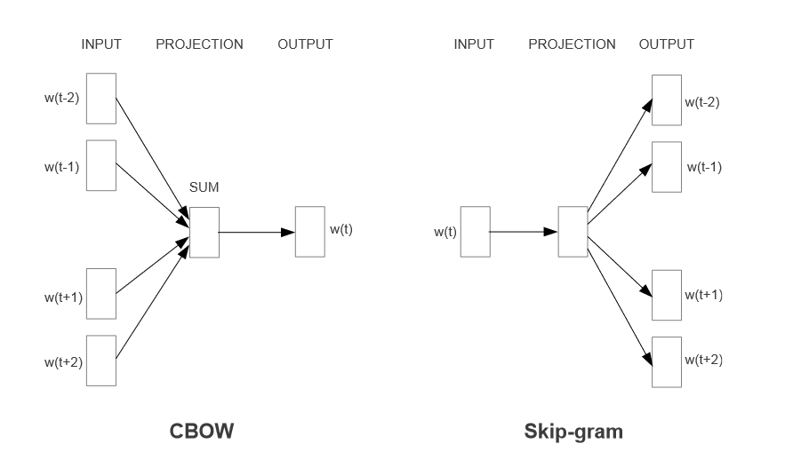
Graphical representation of the CBOW model and Skip-gram model. In the CBOW model, the distributed representations of context (or surrounding words) are combined to predict the word in the middle. In the Skip-gram model, the distributed representation of the input word is used to predict the context. Image source: Exploiting Similarities among Languages for Machine Translation [6].

Further Reading

• Sebastian Ruder’s (https://ruder.io/) second post in a larger series https://ruder.io/word-embeddings-softmax/index.html [7]. See also the first (https://ruder.io/word-embeddings-1/) [8] and third (https://ruder.io/secret-word2vec/) [9] in this series.
• Nice image illustrating Hierarchical Softmax and up-to-date papers on it at Papers with Code: https://web.archive.org/web/20250505064345/https://paperswithcode.com/method/hierarchical-softmax.
• Lei Mao Hierarchical Softmax https://leimao.github.io/article/Hierarchical-Softmax/ [10] [Probably already incorporated.]

Related Concepts

• Lei Mao Noise Contrastive Estimation. https://leimao.github.io/article/Noise-Contrastive-Estimation/ [11].
• Lei Mao Entropy, Perplexity and Its Applications. https://leimao.github.io/blog/Entropy-Perplexity/ [12]

References and Notes

Edit Log

• 14 October 2026: corrected the Boltzmann correspondence ($z_i = -\epsilon_i / kT$), the cost of the softmax denominator (linear, not quadratic, in the feature dimension), the statement of the speed-up, the cluster index $k(w)$ and the attention scaling ($\sqrt{d_k}$); temperature controls the entropy, not the variance, of the output distribution.